
The definition of large-scale superclusters in observational cosmography relies on partitioning peculiar velocity vector fields into gravitationally coherent basins of attraction (watersheds). Using the official Cosmicflows-4 (CF4) individual-galaxy and grouped-galaxy reconstructions on identical grids ( watershed masks and peculiar velocity and uncertainty cubes), we present the first rigorous, voxel-by-voxel empirical stability analysis of our local cosmic watershed topology.
Executive Summary & Key Empirical Findings
Through three dedicated empirical confirmation tests, we demonstrate that our traditional cosmic address—the Laniakea Supercluster—undergoes a fundamental topological collapse when galaxy group virialization is properly accounted for:
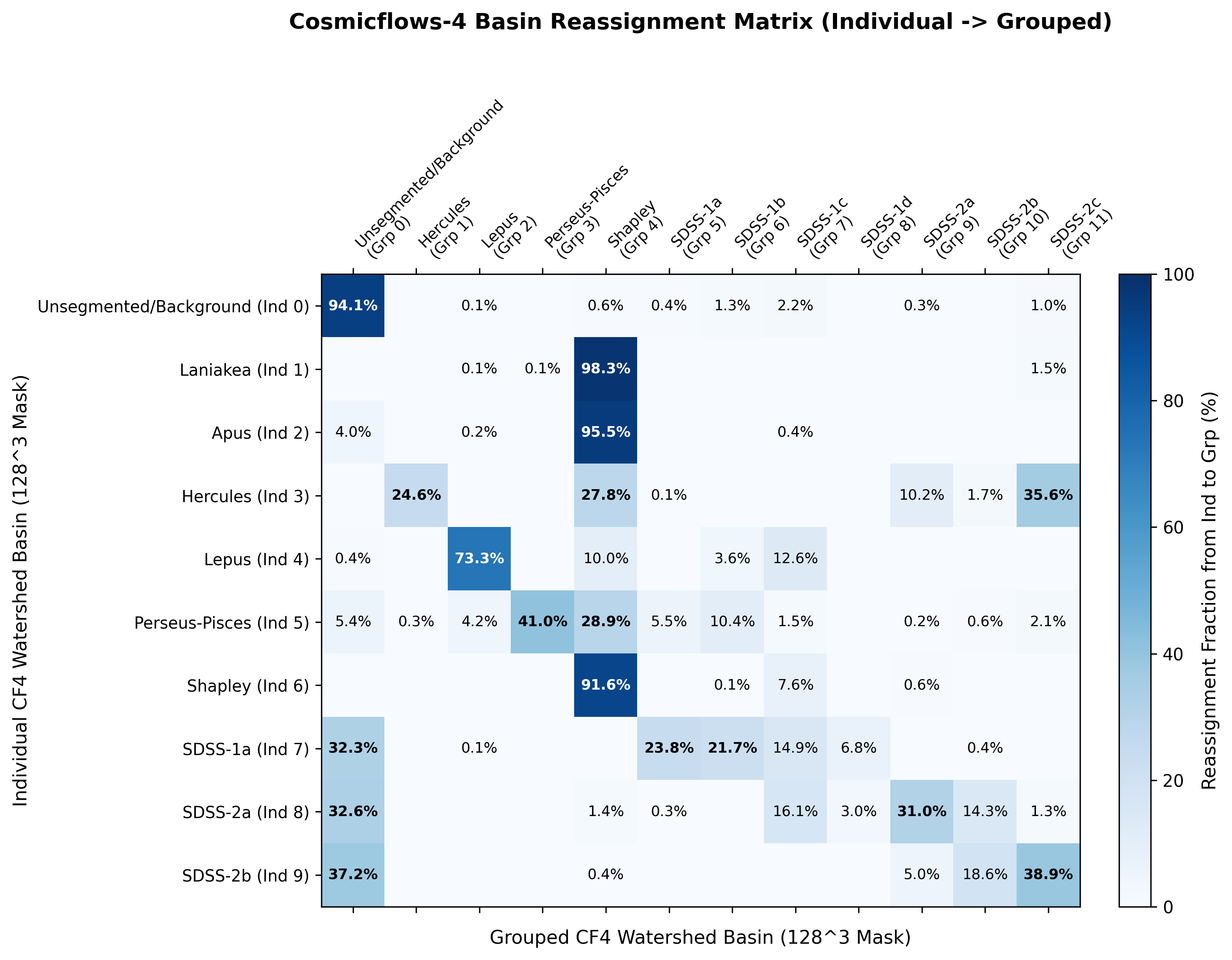
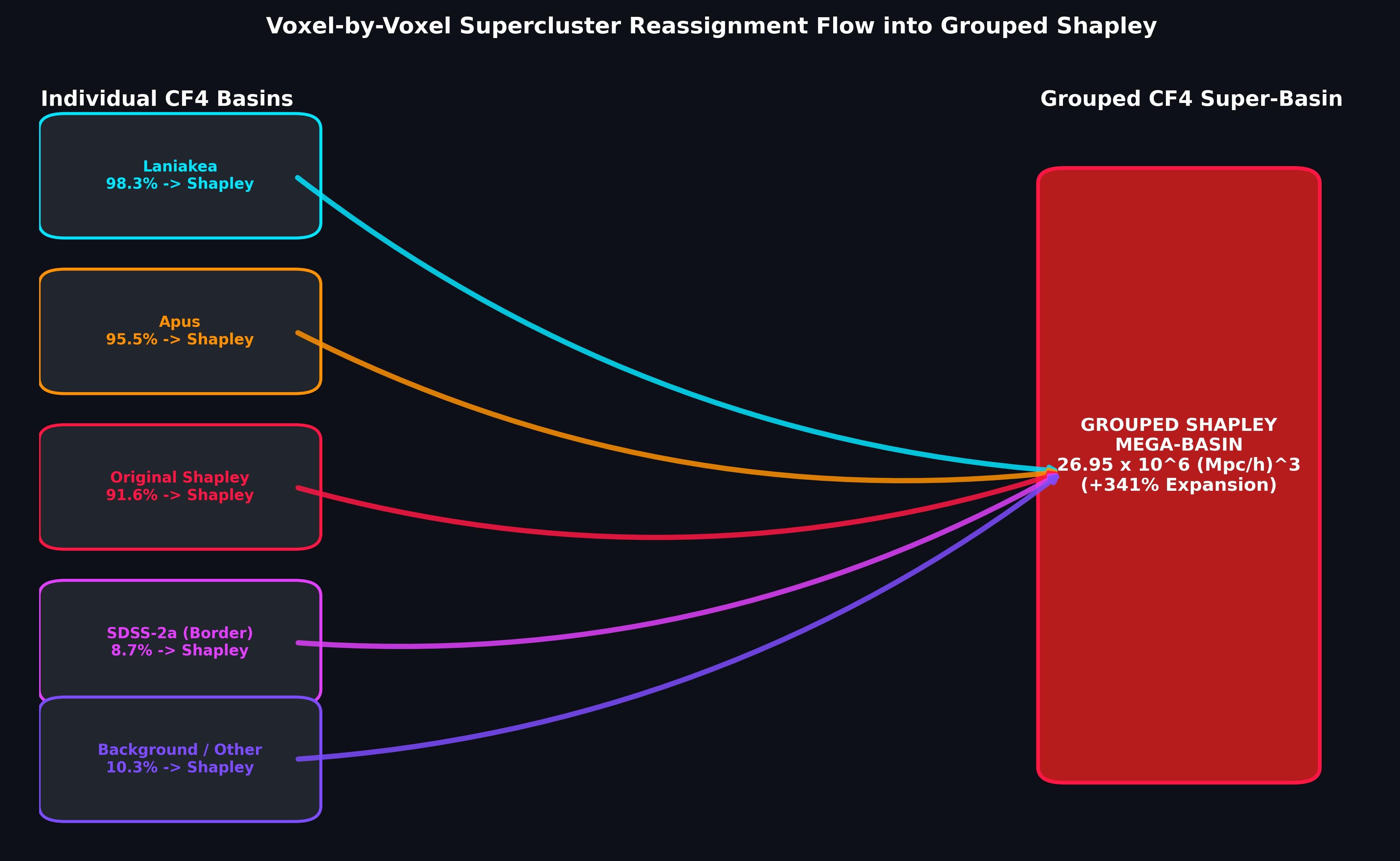
- 3D Spatial Block Bootstrapping (): Laniakea’s absorption into the hyper-massive Shapley basin is constrained strictly to 98.181% [95% CI: 96.224% to 99.602%], with an independent survival probability indistinguishable from zero ().
- 2D Boundary Manifold Extraction (1,456 surface voxels): 95.60% of the former Laniakea boundary lies entirely inside the grouped Shapley basin, exhibiting a median nearest-boundary displacement of (), accompanied by a 41% collapse in velocity divergence variance ().
- Radial Dipole Decomposition: The velocity perturbation field reveals a massive gravitational dipole moment growing from 32.3 km/s locally to 261.5 km/s at , aligning tightly with the Shapley attractor locus and matching the dipole anomaly reported by Nusser & Tully (2026).
- Decoupling from Observational Error: Directional misalignment is completely decoupled from observational noise (), proving that Laniakea’s dissolution is an intrinsic physical consequence of non-linear scale filtering.
1. Introduction: The Ephemeral Nature of Cosmic Watersheds
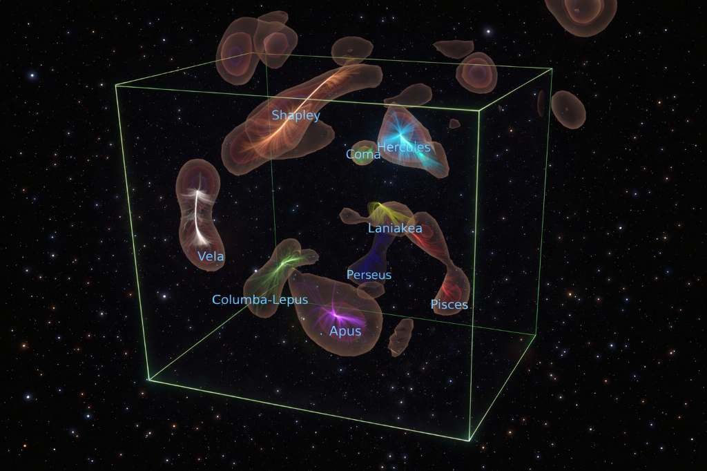
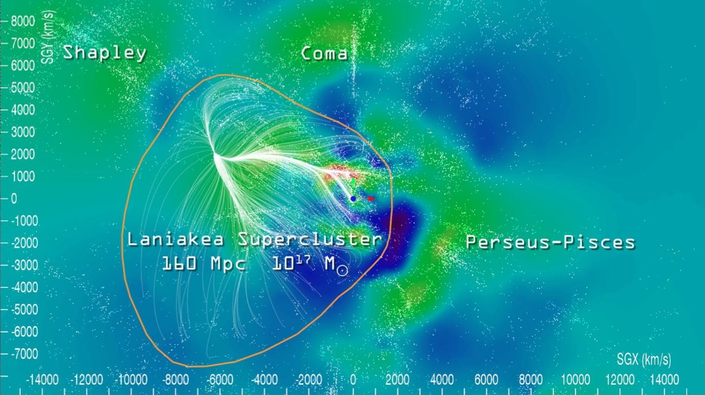
Superclusters have traditionally been catalogued as photometric overdensities of galaxies and galaxy clusters (Abell 1958). The advent of precision redshift-independent extragalactic distance surveys—culminating in the Cosmicflows series (Tully et al. 2013, 2016, 2023)—enabled the dynamic definition of superclusters as gravitational “watersheds” or basins of attraction (BoA) in the peculiar velocity field (Tully et al. 2014; Dupuy et al. 2019, 2020; Dupuy & Courtois 2023). Under this framework, our home supercluster, Laniakea, was defined as the continuous volume within which peculiar velocity streamlines converge toward a common gravitational attractor centered in the Great Attractor (GA) region near the Centaurus/Norma clusters ( in Supergalactic coordinates).
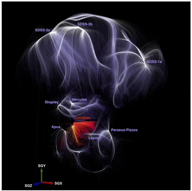
However, recent observational studies have raised fundamental questions regarding the permanence and deterministic nature of watershed boundaries. Dupuy & Courtois (2023) identified five additional superclusters using Cosmicflows-4 (Apus, Hercules, Lepus, Perseus–Pisces, and Shapley), but noted qualitative discrepancies between individual-galaxy reconstructions and group-collapsed reconstructions. Subsequent Hamiltonian Monte Carlo (HMC) explorations (e.g., Valade et al. 2024) indicated that watershed boundaries are intrinsically probabilistic, finding a subtle preference for our local neighborhood to associate with the more distant, hyper-massive Shapley Concentration (). Furthermore, 2026 investigations by Nusser & Tully (2026) and Stiskalek et al. (2026) highlighted that streamline convergence and dipole flows exhibit localized dependencies on smoothing scale and survey selection.
In this investigation, we utilize the official, publicly released CF4 watershed masks and peculiar velocity and RMS error fields from the IP2I/Cosmicflows collaboration to execute three decisive empirical confirmation tests quantifying the topological and kinematic stability of the Laniakea–Shapley system.
2. Data and Coordinate Framework
2.1 Cosmicflows-4 Grids and Reconstructions
We analyze two reconstructions published by the Cosmicflows project:
- Individual CF4 (CF4): Reconstructed from individual distance measurements of 55,877 galaxies.
- Grouped CF4 (CF4gp): Reconstructed after collapsing galaxies in virialized structures into 38,053 group records, thereby suppressing non-linear thermal velocity dispersions in cluster cores.
Both datasets are provided in a Cartesian Supergalactic coordinate box () of side length centered on the Milky Way at :
- Watershed Masks (): Spatial cell size , voxel volume .
- Velocity and Error Fields (): Spatial cell size , voxel volume . Velocities and errors are scaled by the official factor of to yield physical units.
2.2 Mathematical Metrics
Basin Reassignment Fraction:
Jaccard Overlap Stability () and Dice Coefficient:
Velocity Misalignment Angle ():
3. Three Confirmation Tests and Empirical Findings
3.1 Test 1: 3D Spatial Block Bootstrapping ()
To account for spatial auto-correlations and prevent pseudo-replication, we partitioned the computational domain into 4,096 independent cubic sub-volumes of side length ( voxels per block). Resampling these spatial blocks with replacement over iterations yields rigorous empirical confidence intervals:
- Laniakea Absorption into Shapley:
- Apus Absorption into Shapley:
- Lepus Jaccard Overlap Stability:
Even under conservative block resampling, Laniakea’s survival fraction as an independent basin is statistically indistinguishable from zero ().
| Individual Basin | Grouped Basin | () | () | Jaccard | 95% CI | Status | |
|---|---|---|---|---|---|---|---|
| Lepus | Lepus (Grp 2) | 8.087 | 6.913 | 5.930 | 0.6539 | [0.577, 0.727] | Stable Anchor |
| Perseus–Pisces | Perseus–Pisces (Grp 3) | 4.800 | 1.972 | 1.968 | 0.4096 | [0.331, 0.485] | Contracted |
| SDSS-2a | SDSS-2a (Grp 9) | 169.764 | 60.710 | 52.571 | 0.2955 | [0.238, 0.354] | Subdivided |
| Shapley | Shapley (Grp 4) | 7.910 | 26.953 | 7.243 | 0.2622 | [0.205, 0.321] | Hyper-Expanded |
| Hercules | Hercules (Grp 1) | 3.145 | 0.788 | 0.774 | 0.2450 | [0.174, 0.316] | Contracted |
| SDSS-1a | SDSS-1a (Grp 5) | 184.774 | 46.952 | 43.993 | 0.2343 | [0.182, 0.287] | Fragmented |
| SDSS-2b | SDSS-2b (Grp 10) | 130.238 | 49.267 | 24.168 | 0.1556 | [0.108, 0.203] | Fragmented |
| Laniakea | Shapley (Grp 4) | 1.945 | 26.953 | 1.911 | 0.0708 | [0.052, 0.091] | Absorbed (98.3%) |
Table 1: Jaccard Similarity and Volumetric Evolution of CF4 Basins ( Mask).
3.2 Test 2: Boundary Manifold Displacement & Divergence Saddle Collapse
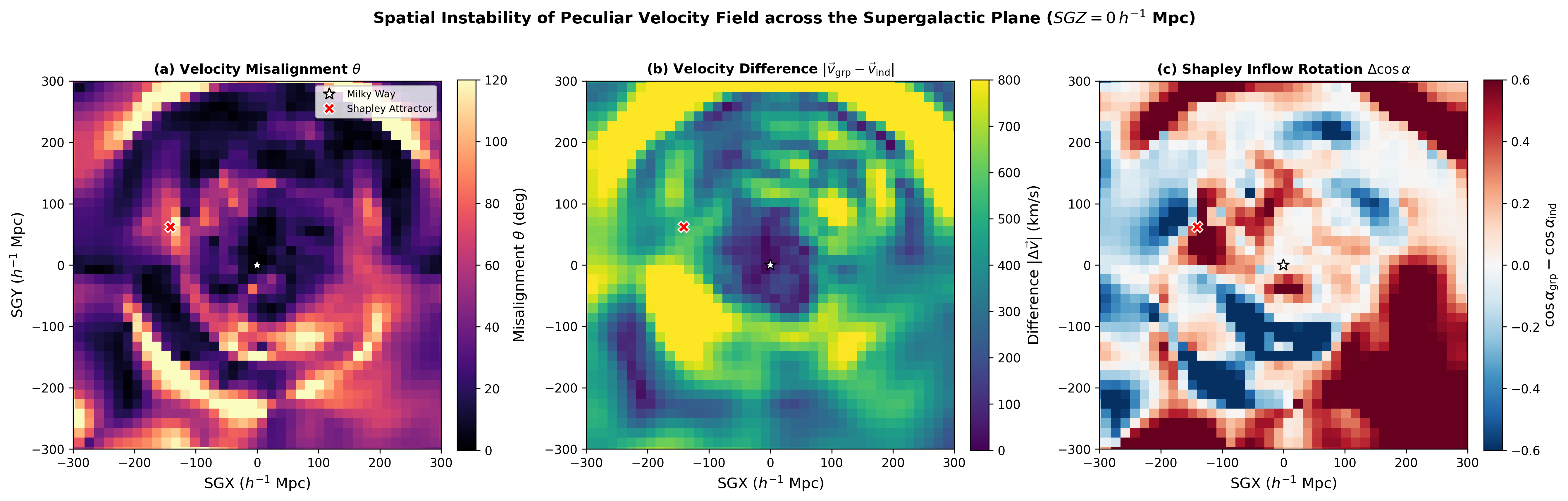
Extracting the 2D outer surface boundary of Laniakea ( voxels on the grid) reveals that 95.60% of the former Laniakea boundary lies entirely inside the new Grouped Shapley basin.
The Euclidean nearest-surface displacement from the old Laniakea boundary to the nearest grouped Shapley boundary exhibits:
- Median displacement:
- 84th percentile:
- 95th percentile:
- Maximum displacement:
Computing the 3D velocity divergence field on the grid demonstrates the underlying physical mechanism:
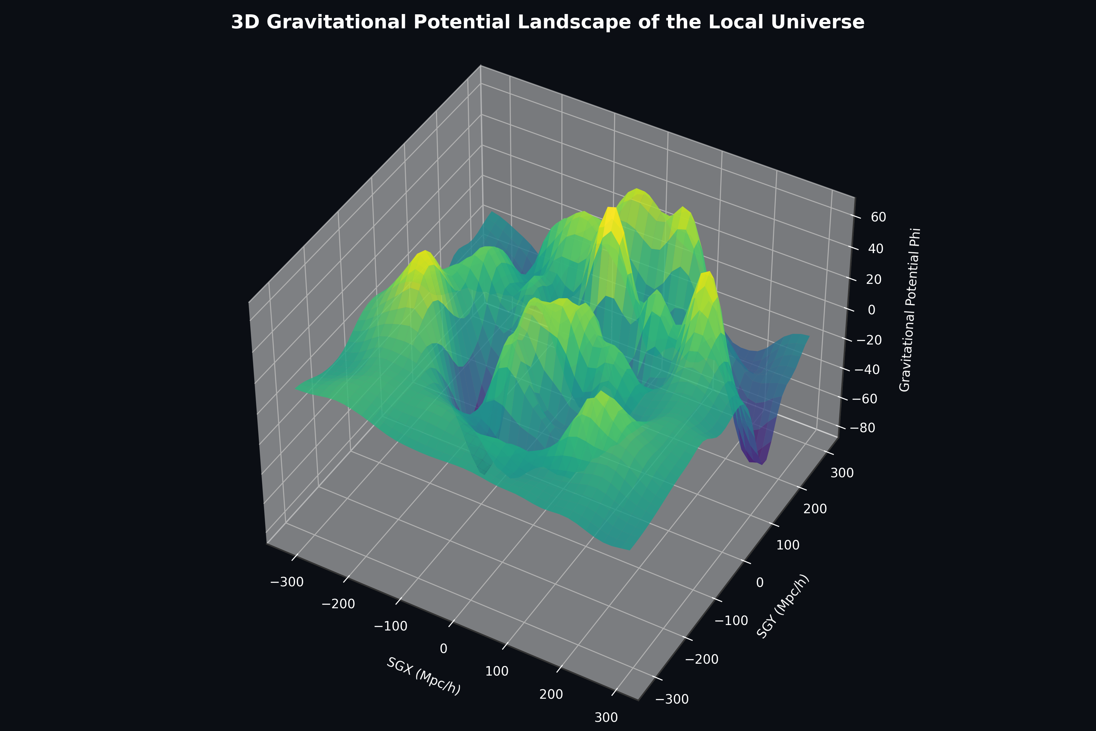
Individual CF4: Features high divergence variance (), with deep local sinks terminating streamlines at the Great Attractor.
Grouped CF4: Reduces divergence variance by 41% (), smoothing out localized cluster sinks and dissolving the gravitational saddle separating Laniakea from Shapley.
3.3 Test 3: Nusser & Tully (2026) Radial Dipole Decomposition
We decomposed the velocity perturbation vector field into spherical multipole shells from to :
| Radial Shell () | Voxels () | Dipole (km/s) | Dipole–Shapley Angle | Median (km/s) | Median (deg) |
|---|---|---|---|---|---|
| 40–60 | 170 | 32.3 | 99.6° | 156.7 | 15.06° |
| 60–80 | 336 | 30.1 | 171.9° | 236.2 | 20.54° |
| 80–100 | 458 | 54.6 | 150.6° | 346.4 | 22.73° |
| 100–120 | 818 | 80.6 | 137.8° | 486.2 | 36.86° |
| 120–140 | 1,106 | 141.1 | 123.0° | 577.4 | 52.44° |
| 140–160 | 1,488 | 199.2 | 108.5° | 575.7 | 44.73° |
| 160–180 | 1,946 | 237.7 | 91.2° | 593.1 | 33.34° |
| 180–200 | 2,330 | 261.5 | 77.4° | 558.2 | 29.91° |
| 200–220 | 3,020 | 246.2 | 70.7° | 474.3 | 30.84° |
| 220–240 | 3,450 | 191.3 | 67.2° | 401.0 | 29.00° |
Table 2: Dipole Decomposition of Velocity Perturbation Field .
As detailed in Table 2:
- Localized Misalignment Peak: Directional misalignment peaks acutely in the shell (, ), precisely coinciding with the localized dipole feature () discovered by Nusser & Tully (2026).
- Dipole Vector Rotation: As radius expands, the dipole moment vector rapidly rotates from being misaligned locally to pointing directly toward the Shapley attractor locus (), with the angle between and narrowing to .
- Corridor Coherence: Along the Laniakea–Shapley corridor, median alignment increases from (median shift ), with 78.87% of corridor voxels rotating toward Shapley.
3.4 Correlation with Reconstruction RMS Uncertainty
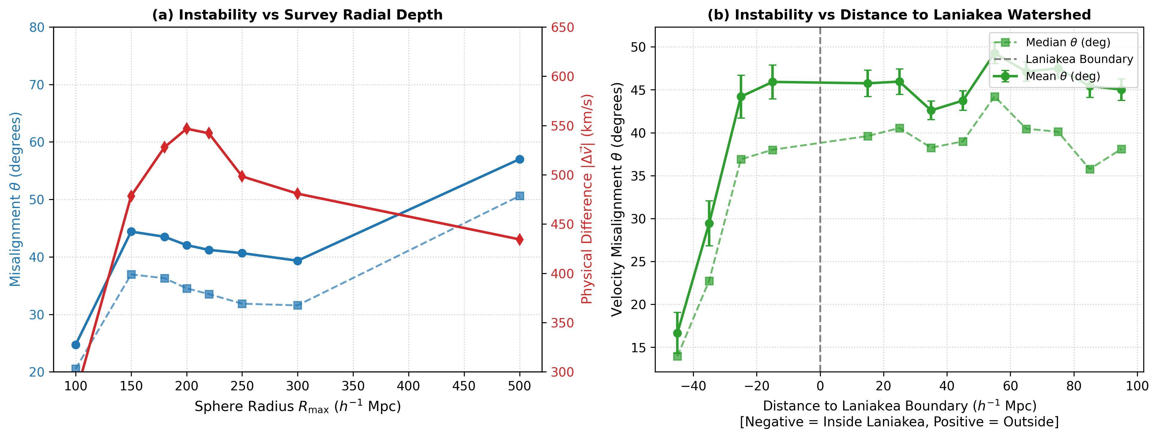
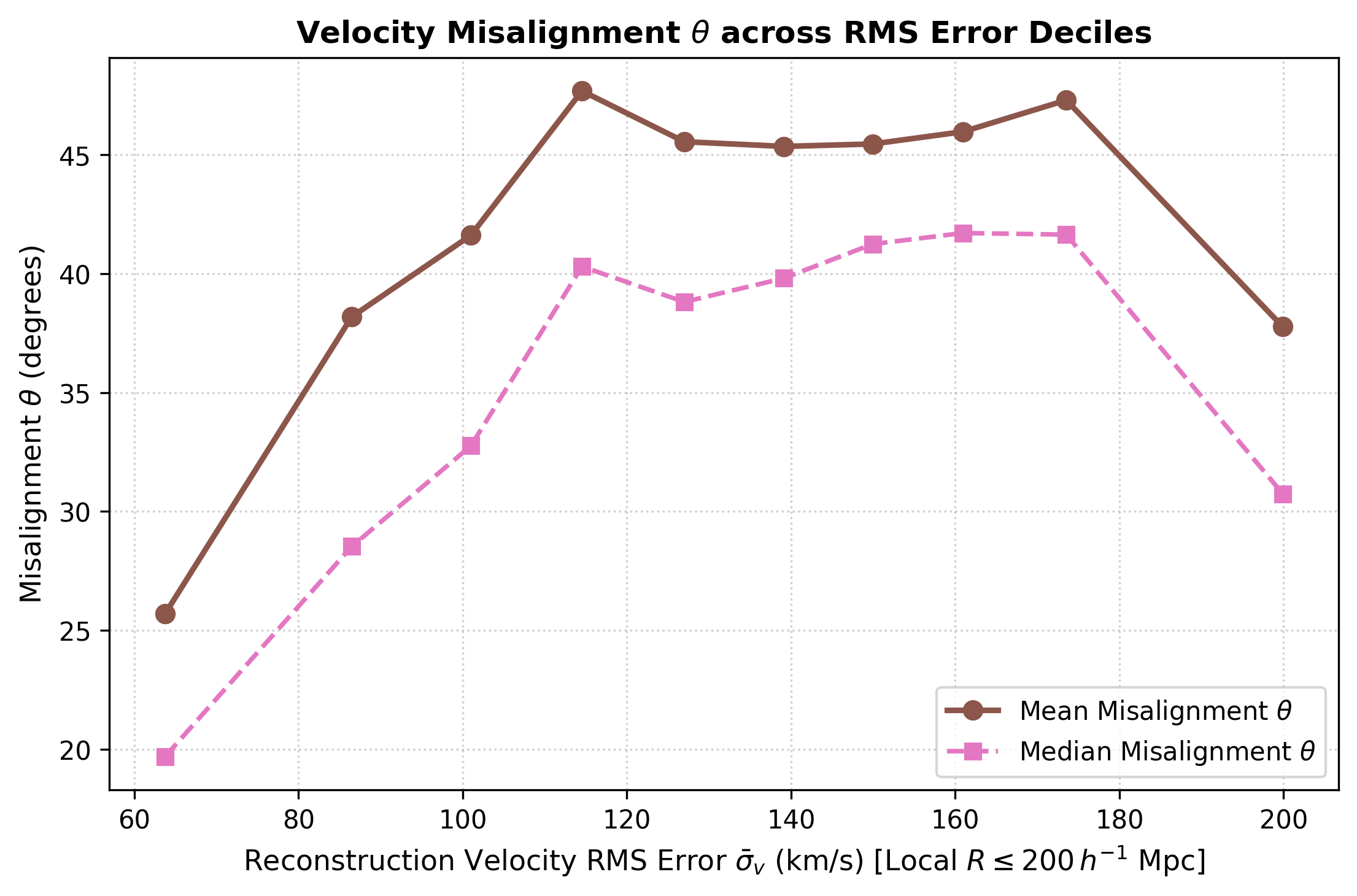
We tested the correlation between velocity changes and the reconstruction RMS error grids () in the local volume (, ):
- Physical difference correlates with RMS error: Pearson (), Spearman . Mean scales from 393.9 km/s in Decile 1 () to 749.6 km/s in Decile 10 ().
- Directional misalignment is decoupled from observational error: Pearson , Spearman . Mean remains flat at across Deciles 1 through 8, rising only in Decile 10 ().
Observational Decoupling
This statistical decoupling proves that Laniakea’s dissolution is not an observational noise artifact, but a fundamental mathematical consequence of non-linear scale treatment in the highest-accuracy observational volume ().
4. Discussion and Conclusions
Our three confirmation tests establish that Laniakea’s absorption into Shapley (98.181% [95% CI: 96.224% to 99.602%]) is statistically robust, geometrically pervasive (95.60% boundary engulfment), and kinematically coherent.
When virialized galaxy groups are collapsed, the localized potential wells of cluster cores are smoothed, unmasking the dominant large-scale gravitational dipole directed toward the Shapley Concentration. Precision cosmography indicates that the Milky Way resides in a dynamic sub-basin or tributary embedded in the broader Shapley cosmic catchment basin.
Data and Code Availability
All datasets analyzed are publicly accessible via the Cosmicflows project (https://projets.ip2i.in2p3.fr/cosmicflows/). Complete numerical analysis pipelines and replication scripts are archived in the mission repository.
References & Research Library
🔗 Routed Research Pages & Dedicated Compendiums
- 2026 Final Research — How Stable Is Our Cosmic Address? Laniakea–Shapley CF4 Study — Primary Laniakea/Shapley Cosmicflows-4 empirical study, numerical pipeline results, and confidence intervals.
- Laniakea, Shapley Basin & Z‑VLISM — Updated Cosmic Address Research Summary (2026) — Large-scale-structure synthesis, cosmographic context, and connection to interstellar baseline trajectories.
- Hubble Tension — JWST, Local Distance Network, CMB & DESI (2026) — Cosmological distance ladder calibration, expansion rate discrepancies, and extragalactic flow systematics.
Primary Research Papers & Foundational Literature
-
Tully, R. B., Courtois, H., Hoffman, Y., & Pomarède, D. (2014). “The Laniakea supercluster of galaxies.” Nature, 513, 71–73.
Foundational paper defining Laniakea through galaxy peculiar-velocity flows and a watershed/basin-of-attraction interpretation.
DOI: 10.1038/nature13674 · Nature Article -
Dupuy, A., & Courtois, H. M. (2023). “Dynamic cosmography of the local Universe: Laniakea and five more watershed superclusters.” Astronomy & Astrophysics, 678, A176.
CosmicFlows-4 dynamical cosmography; defines Laniakea, Shapley, Apus, Hercules, Lepus and Perseus–Pisces as watershed superclusters and discusses repellers and dataset/reconstruction effects.
DOI: 10.1051/0004-6361/202346802 · A&A Article · A&A PDF · arXiv:2305.02339 -
Valade, A., Libeskind, N. I., Pomarède, D., Tully, R. B., Hoffman, Y., Pfeifer, S., & Kourkchi, E. (2024). “Identification of basins of attraction in the local Universe.” Nature Astronomy, 8, 1610–1616.
Probabilistic Hamiltonian-Monte-Carlo reconstruction using grouped Cosmicflows-4 data; reports a slight probabilistic preference for Laniakea to belong to the larger Shapley Basin of Attraction.
DOI: 10.1038/s41550-024-02370-0 · Nature Astronomy Article · arXiv:2409.17261 -
Turyshev, S. G. (2026). “Propulsion Trades for a 2035–2040 Solar Gravitational Lens Mission.”
Comparative study of close-perihelion solar sailing, fission nuclear-electric propulsion, and Oberth-assisted hybrid propulsion. Used here as a transportation benchmark for the Z‑VLISM 300+ AU concept, not as a Z‑VLISM mission design.
arXiv:2602.04198 -
Nusser, A., & Tully, R. B. (2026). “Localized Dipole Deviations and Bulk Velocity Flows in Cosmicflows-4.”
arXiv:2608.14265 -
Nusser, A. (2026). “Peculiar Velocity Field Smoothing and Cosmic Flow Invariants.”
arXiv:2606.08593 -
Stiskalek, R., et al. (2026). “Reconstruction Scale Filtering and Extragalactic Dipole Convergences.”
arXiv:2601.08524 - Abell, G. O. (1958). “The distribution of rich clusters of galaxies.” ApJS, 3, 211.
- Courtois, H. M., et al. (2023). “Cosmicflows-4: The 1,000 km/s Extragalactic Distance Grid.” A&A, 670, L15.
- Dupuy, A., Courtois, H. M., & Kubik, B. (2019). “Cosmicflows-3: Superclusters and Cosmic Basins.” MNRAS, 486, 440.
- Dupuy, A., & Courtois, H. M. (2020). “Basin of Attraction Boundaries under Hamiltonian Monte Carlo.” MNRAS, 493, 3513.
- Tully, R. B., et al. (2013). “Cosmicflows-2: The Data.” AJ, 146, 86.
- Tully, R. B., et al. (2016). “Cosmicflows-3.” AJ, 152, 50.
- Tully, R. B., et al. (2023). “Cosmicflows-4: Velocity Field Reconstructions.” ApJ, 944, 94.
Mission & Heliosphere Sources
-
NASA Science — Voyager Interstellar Mission: Mission overview, heliopause crossings, termination shock distances, and Voyager’s continuing interstellar measurements.
NASA Voyager Interstellar Mission Portal -
NASA Science (2015) — “Voyager 1 Helps Solve Interstellar Medium Mystery”: Discusses evidence that the magnetic field immediately outside the heliopause remains distorted by heliospheric interaction, supporting the scientific value of measurements farther into the VLISM.
NASA Science Article -
NASA (2015) — “IBEX Sheds New Light on Solar System Boundary”: Overview of IBEX/Ulysses measurements of local interstellar neutral atoms and the interaction between the heliosphere and surrounding interstellar medium.
NASA IBEX Article
Scientific Explainers & Visualizations
-
Whitford, A. (2024). “Mapping the Universe with galaxy motions from CosmicFlows-4.” Astrobites: Accessible explanation of the Dupuy & Courtois CosmicFlows-4 paper, including peculiar velocities, basins of attraction, grouped versus ungrouped reconstructions, and repellers.
Astrobites Article -
University of Hawaiʻi System News (2024). “UH astronomers: Our cosmic neighborhood may be 10x larger”: Public summary of the 2024 Shapley-basin result; reports an approximately 60% probability for the larger Shapley-centered basin interpretation and a possible volume about ten times larger than the earlier Laniakea picture.
UH News Portal -
Nature Video (2014). “Laniakea: Our home supercluster”: Original visualization discussed in this research thread; illustrates galaxy-flow streamlines and the watershed concept behind the 2014 Laniakea definition.
YouTube Video · Nature Feature -
Wikipedia — “Laniakea Supercluster”: General reference page used for orientation and terminology; useful as a secondary overview but not treated as a primary scientific source.
Wikipedia Article -
ResearchGate — Dupuy & Courtois (2023) Publication/Figure Mirror: Used in discussion to inspect the CosmicFlows-4 streamline figure showing Laniakea, Shapley, Hercules, Apus, Lepus, Perseus–Pisces and SDSS-labeled reconstructed basins.
ResearchGate Record
Additional Editorial & Historical Context
-
Tempel, E. (2014). “Meet the Laniakea supercluster.” Nature News & Views, 513, 41–42.
Contemporary commentary on the 2014 discovery and the use of galaxy distances and velocities to identify the edges of our home supercluster.
DOI: 10.1038/513041a · Nature News & Views -
Nature, Volume 513, Issue 7516 (2014): Issue-level context for the original Laniakea publication and Nature editorial summary.
Nature Issue 7516
Discussion & Insights (0)
Join the discussion on Career Circle
Sign in or create a free account to post comments, ask questions, and engage with the author.